
Abstract
The intermodal hinterland transportation of maritime containers is under pressure from port authorities and shippers to achieve a more integrated, efficient network operation. Current optimisation methods in literature yield limited results in practice, though, as the transportation product structure limits the flexibility to optimise network logistics. Synchromodality aims to overcome this by a new product structure based on differentiation in price and lead time. Each product is considered as a fare class with a related service level, allowing to target different customer segments and to use revenue management for maximising revenue. However, higher priced fare classes come with tighter planning restrictions and must be carefully balanced with lower priced fare classes to match available capacity and optimise network utilisation. Based on the developments of intermodal networks in North West European, such as the network of European Gateway Services, the Cargo Fare Class Mix problem is proposed. Its purpose is to set limits for each fare class at a tactical level, such that the expected revenue is maximised, considering the available capacity at the operational level. Setting limits at the tactical level is important, as it reflects the necessity of long-term agreements between the transportation provider and its customers. A solution method for an intermodal corridor is proposed, considering a single intermodal connection towards a region with multiple destinations. The main purpose of the article is to show that using a limit on each fare class increases revenue and reliability, thereby outperforming existing fare class mix policies, such as Littlewood.
1 Introduction
Since 2011, the study of planning models for intermodal container transportation has received much attention, e.g. in Caris et al. (2013), Nabais et al. (2013), SteadieSeifi et al. (2014), Li et al. (2015) and Van Riessen et al. (2015a, 2016). The motivation for this renewed attention is two-fold: optimisation is required to meet the modal split targets in deep sea ports and to satisfy the need for a more integrated approach to hinterland transportation. Firstly, several port authorities have stated modal split targets, e.g. in Rotterdam (Port of Rotterdam 2011), Hamburg and Antwerp (Van den Berg and De Langen 2014). Attaining the modal split levels for port operators necessitates a planning approach that considers multiple modes and routes integrally, we refer to this as an integrated network planning approach. Secondly, several studies recognised the need for such an integrated approach for several stakeholders in container supply chains, e.g. Franc and Van der Horst (2010), Veenstra et al. (2012) and Top Sector Logistics (2011). Available network optimisation models mostly assume that all transportation orders can be scheduled with full flexibility, considering operational constraints and time windows. However, integral network optimisation models have limited value as long as no integral coordination is possible. The need for a differentiated product portfolio was described in Van Riessen et al. (2015b). Ypsilantis (2016, pp. 23–46) showed that container dwell times at terminals largely depend on shipper’s actions, representing a varying need of urgency of further transporting containers. This relates to a high variation in the number of transports from day to day, as shippers generally order for transportation with a fixed mode, route and time. Such orders do not give the operator of an inland transportation network any flexibility for integral optimisation. Some flexibility, allowing the network operator to choose from multiple options per order, could be used to optimise the network transportation plan. Therefore, the network operator has an incentive to introduce a range of transportation services with varying levels of flexibility. Such new product ranges have been studied at EGS by Lin (2014) and independently by Wanders (2014). Their work is related to the development of differentiated product portfolios in practical applications in North West Europe, such as in the hinterland transportation network of European Gateway Services (see European Gateway Services, n.d.). EGS is considering to offer a differentiated portfolio to the market, starting with a single corridor in its network. Their goal is to increase both utilisation of inland trains and vessels, and to increase reliability of container transports arriving on time. In this article, we study their case to find the benefit of a new set of two products with a different degree of flexibility for a single corridor of container hinterland transportation. We compare corridors, based on differences in demand and price levels to support EGS in deciding which corridor is most promising. The new portfolio consists of two fare classes with varying delivery lead times and prices. In a traditional capacity allocation model, typically the inferior fare class is limited, to reserve space for the superior fare class with high revenue (such as Littlewood 1972/2005). In the EGS case however, long-term commitments to customers with repetitive demand are made, and all incoming demand for a fare class within the commitment must be transported. To achieve an optimal balance between both fare classes, a limit for each fare class must be determined. This is a problem similar to the fare mix problem in aviation: how much available capacity must be reserved for each fare class? The main purpose of this article is to show how offering two fare classes can significantly increase revenue compared to alternative approaches. Also, we show that including limits for each fare class is not only necessary to prevent high costs of trucking excess cargo, it is even beneficial in terms of expected revenue compared to alternatives. We define these problems as the Cargo Fare Class Mix (CFCM) problem. This class of problems is based on differentiated service portfolios in intermodal networks, but it is also relevant for applications in parcel delivery services and inventory management in online retail. We provide a framework to distinguish between different variants of the problem and we provide analytical solution methods for a single corridor. We propose a model and exact solution method for the special case of the CFCM problem with two products in an application with 1 intermodal route, multiple destinations and a horizon of 2 delivery periods. We demonstrate the model and solution method in a case study of many different parameter settings comparing different hinterland transportation corridors. This case study supports European Gateway Services in introducing such a differentiated portfolio. Finally, we show by numerical experiments that the increase in expected revenue by considering a longer delivery horizon is limited.
The remainder of the article is structured as follows. Section 2 provides an overview of existing literature on intermodal networks and revenue management in freight applications. Section 3 proposes a classification structure for different variants of the CFCM problem and describes the special case of the CFCM problem for a single corridor. Section 4 describes the proposed solution method for this case and Sect. 5 presents a case study and results, showing the potential gains for this case. Section 6 concludes this article with an overview and outlook to future research.
2 Literature review
2.1 Intermodal networks
Supply chains get increasingly interconnected and shippers demand higher levels of service, such as short delivery times and reliability (Veenstra et al. 2012; Van Riessen et al. 2015a). The logistic expression for integrated transportation is intermodality. The main challenge for an intermodal network operator is the continuous construction of an efficient transportation plan. That is, the allocation of containers to available inland services (train, barge or truck). Generally, container hinterland transportation is organised per corridor between a deepsea port and a hinterland destination, although integral network operators are arising, such as EGS (Veenstra et al. 2012). Consolidation of flows between hubs in barge of train services is cost efficient as it benefits from the economies of scale (Ishfaq and Sox 2012). For a complete overview on intermodal planning optimisation, see SteadieSeifi et al. (2014). The approach towards offering hinterland transportation services is changing. Franc and Van der Horst (2010) studied the motivation of shipping lines and terminals for the integration of the hinterland in their service. Veenstra et al. (2012) introduced the concept of extended gates for deep sea terminals. Currently, many studies refer to the concept of synchromodal transportation (e.g. Top Sector Logistics 2011; SteadieSeifi et al. 2014; Behdani et al. 2016), aiming for real-time optimal transportation planning in an integrated hinterland transportation system. Synchromodality can only really provide an advantage if the intermodal planning problem is considered in conjunction with the product portfolio offered to customers (Van Riessen et al. 2015b). Related to this, some researchers have studied the pricing problem of intermodal inland services. Ypsilantis (2016, pp. 47–82) proposed a model for jointly determining prices for transportation products and designing the transportation network. Li et al. (2015) study the problem of pricing a differentiated portfolio in a cargo network based on expected realised costs, considering the network state. These works have not looked into the optimal fare class mix of offered transportation services yet, though.
2.2 Revenue management in freight transportation
The concept of different service propositions in transportation is very similar to the concept of different fare classes for the same flight in aviation. Barnhart et al. (2003) give an overview of operations research in airline revenue management. The primary objective of airline revenue management models is to determine the optimal fare mix: how many seats of each booking class should be available, given demand forecasts and a limited total number of seats? Some studies on revenue management in freight transportation focus on the online policy: whether to accept or reject an incoming order. Pak and Dekker (2004) propose a method for judging sequentially arriving cargo bookings based on expected revenues. If the direct revenue of a booking exceeds the decrease in expected future revenue, the order is accepted. Bilegan et al. (2013) apply a similar approach on rail freight application. In their approach the decision of accepting or rejecting an arriving transport order is based on the difference in expected revenue with and without that order. These studies assume that accepting or rejecting an incoming order can be done at the operational level. Other studies acknowledge that in freight transportation orders are often agreed on in long-term contracts. Because of this, a per-order approach to revenue management is not sufficient. The traditional revenue management approach is to reserve capacity at the tactical level for a superior service, while the remainder of the capacity is offered at the operational level (Chopra and Meindl, 2014). Liu and Yang (2015) develop a two stage stochastic model for this problem: in the first stage, all long-term contracts are accommodated; in the second stage a dynamic pricing model is applied for offering the remaining slots. In all these studies, it is assumed that the planning characteristics of all orders are identical, i.e. an order of any service can be carried out with the same transportation options.
To our knowledge, no existing studies have looked into the Cargo Fare Class Mix of differentiated services with different planning characteristics. In this study we aim to determine the optimal cargo fare mix for a given service portfolio with difference in both price and leadtime. This setting introduces a new issue to the fare mix problem, as the operator must balance between higher priced service with few transportation options and lower priced services with more transport options (e.g. different modes, routes and times). Hence, a lower priced service allows more flexibility in the operational plan and is not simply inferior to a higher priced service. As transportation orders for each service type are agreed on in long-term contracts, an optimal mix between the offered services must be determined in advance, at the tactical level. Besides, all demand accepted at the tactical level must be transported; if intermodal capacity is insufficient, a high cost truck transport is needed for the excess demand. Hence, we must determine fare class limits for all services, not only for the lower priced service.
3 Cargo Fare Class Mix problem
3.1 Practical motivation
In the CFCM problem, as we define it, the transportation provider’s goal is to maximise revenue by finding the optimal balance in offered transportation services. The transportation provider runs scheduled intermodal connections with a fixed daily capacity. The transportation provider offers a range of two or more services, each service denotes a fare class. A fare class is characterised by a specific price and specific lead time, ranging from a high price fast service to a low price slow service. For instance, the fast service pays more per container, but must be transported immediately; whereas the slow service pays less, but has a longer delivery lead time and allows optimising the capacity utilisation, because demand varies over the days. It is assumed that using the available capacity does not invoke additional costs. This corresponds to a company operating its own trains or vessels. As a lower priced service offers more planning flexibility, it is not necessarily inferior to a higher priced product. All accepted demand must be transported, because of commitments to the customer and if the intermodal capacity is not enough, expensive trucking is used. Hence, an optimal balance requires a booking limit for each fare class. As discussed in the Literature review, this is different from traditional cargo revenue management, in which only one (inferior) fare class is limited. Another distinct difference with existing literature is that accepting or rejecting incoming orders cannot be decided on during the operational phase, because long-term commitments are provided in advance and customers typically have a repeating demand. To represent long-term commitments in our model, we consider daily booking limits, determined on a tactical level (before the operational phase). With fixed booking limits for each service, the operator can optimally use his fixed transportation capacity to target different segments allowing revenue maximisation. We will show that it is better to allow overbooking, or in other words, the sum of the booking limits may exceed the daily intermodal capacity, as for the lower class we have the option to transport it later. The general CFCM problem must accommodate fare classes for transportation services to multiple inland destinations considering a transportation network. In this article, we demonstrate the benefit of booking limits for each fare class on a single intermodal corridor, with one intermodal route, e.g. a train connection between the deep sea port (like Rotterdam) and an inland terminal (such as Venlo). In the next sections, we first present a general modelling framework for the CFCM problem, after which we define the specific model for such a single corridor for our study.
3.2 Modelling framework
The CFCM problem for inland transportation has three dimensions. The tactical planning problem considers multiple routes r and destinations d for transporting all cargo. Because the intermodal transportation problem is mostly related to one deep sea port, we do not distinguish between multiple origins. Transportation orders arrive in multiple fare classes; the number of fare classes p is the third dimension. We use the 3 dimensions to classify the problem type of the CFCM problem as CFCM (r, d, p), as shown schematically in Fig. 1. Each fare class is associated with a maximum transportation time. In the tactical problem we define booking limits for each class. In the repetitive operational problem, incoming transportation requests for a fare class are accepted up to the booking limit for that fare class. It is assumed that all orders arrive one by one. Then, the operational transportation plan for all accepted orders is created, assigning to each order a route towards the destination or postponing the order to the next period. After executing the transportation plan, we continue with the next period. The goal of the operational transportation plan is to minimise costs within capacity restrictions and to transport all accepted orders within the time limits related to the fare class ordered by the customer. In this article, we study the CFCM problem of a single corridor, providing insights to be used as a building block for future extensions.

Schematic model of the Cargo Fare Class Mix problem with r intermodal routes, d destinations and p fare classes, CFCM (r, d, p)
3.3 CFCM problem for an intermodal corridor
To show the benefits of the CFCM model with limits for each fare class, we consider a single intermodal corridor with two products in this article. Such a case is representative of a typical intermodal hinterland corridor between a deep sea port and a hinterland terminal. Inland transportation providers such as EGS are currently considering to offer a Standard and Express service types on such a corridor but do not have insight in the optimal balance yet. First, we will focus on daily booking limits for two services for a single route, single destination case, and derive a solution for the CFCM (1, 1, 2) model (Fig. 2). Subsequently, we consider the case of two fare classes for a single route, with multiple destinations, the CFCM (1, d, 2) model (Fig. 3). In the latter case, the costs of using a truck to transport Excess demand varies for different destinations. With some realistic assumptions, we show that the CFCM (1, 1, 2) model can be applied to CFCM (1, d, 2) as well. For this, we assume that using the intermodal connections is beneficial for all destinations considered, compared to the alternative, direct trucking. Also, we assume that the difference in distance for the various destinations is relatively small, compared to the total distance and that the amount of cargo is distributed over all destinations.

Schematic model of the Cargo Fare Class Mix problem with 1 route, 1 destination and 2 fare classes, CFCM (1, 1, 2)

Schematic model of the Cargo Fare Class Mix problem with 1 route, d destination and 2 fare classes, CFCM (1, d, 2)
We derive an analytical model for the CFCM (1, 1, 2) problem with daily booking limits. This model’s focus is on optimising revenue from 2 product types, Express and Standard, for a fixed capacity C on one route to one destination. In case of Express transportation, the container is transported within 1 day. For Standard transportation, the container is transported within 2 days. At the tactical level, the available demand (not restricted by booking limits) of daily transportation requests is assumed to be characterised by discrete distributions N E(t) and \( N_{\text{S}} \left( t \right) \), with subsequent days i.i.d. Also, we assume N E(t) and \( N_{\text{S}} \left( t \right) \) are mutually independent and having different distributions,
where \( p_{\text{E}} \left( k \right) \) denotes the probability of receiving k transportation requests for fare class \(E\) on a day. It is assumed that the demand on consecutive days for a fare class follows identical, independent distributions. Transportation requests on a daily basis for a fare class are accepted until the booking limit for that fare class is reached, the remaining demand is assumed lost. For carrying out the transportation, the operator has a daily transportation capacity C that can be used for service requests of type E and/or S. Excess demand that cannot be transported in time on daily capacity C must be transported by using an (expensive) truck move. This must be avoided, so in order to prevent accepting too many requests, the operator only accepts demand up to the daily booking limits for both request types: L E and L S. With this, the distributions of daily accepted demand become:
and, likewise,
In the remainder, the indicator (t) is omitted from the notation for simplicity, unless specifically required for clarity. It is assumed that the accepted demand of type E is given priority, as, by agreement, the orders of type S can be postponed to the next day. It makes no sense to accept more Express orders than the capacity limit, because the amount of orders exceeding C cannot be transported with the available capacity, i.e. L E ≤ C. Hence, every day, all accepted demand of type E is transported, denoted by T E. The remaining capacity is used for transporting accepted demand of type S; the transported amount of type S is denoted by T S. On any day, the stack of orders to be transported consists of three types: today’s accepted demand of type E (D E), the remainder of yesterday’s demand of type S (R S) and today’s demand of type S (D S). The demand D S of today that is not transported, is considered on the next day, denoted as R S(t + 1). If the postponed demand R S(t + 1) cannot be transported the day after, it is considered as excess demand (E S). Three situations can occur:
-
1.
The available capacity is sufficient for transporting D E and part of R S (see Fig. 4a), the remainder of R S is in excess of capacity C and must be transported alternatively (E S);
Fig. 4 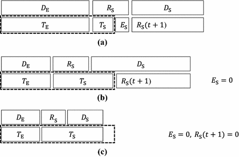
Transportation plan based on fixed capacity (3 situations). a Result situation 1: transported, excess and remaining, b result situation 2: transported and remaining, c result situation 3: all demand transported
-
2.
The available capacity is sufficient for transporting D E, R S and part of \( D_{\text{S}} \) (see Fig. 4b);
-
3.
The available capacity is sufficient for transporting all demand (see Fig. 4c).

The revenue maximising problem is to select booking limits that maximise the total revenue J from the accepted demand, with fares per accepted request f E and f S respectively, while considering a penalty of size p for all excess demand. This penalty can be considered as the costs for an emergency delivery outside of the system’s capacity C:
The cost term for excess demand distinguishes this model from existing problems, as transportation of the accepted Standard product is obligatory as well. The expected Excess \( {\mathbb{E}}\left( {E_{\text{S}} } \right) \) depend on the booking limits L E, L S and in the next section we will derive the formulation for this quantity.
4 Solution method for the CFCM problem for an intermodal corridor
For solving (4), we first derive a set of equations for the expected value of D E, D S and E S as a function of capacity C and the booking limits L E and L S. These expressions are then used to find the booking limits L E and L S that result in maximum revenue J.
The distributions of accepted demand D E, \( D_{\text{S}} \) depend according to (1) only on the independent demand patterns N E and N S (assumed to be known) and on the chosen limits L E and L S. Formulations for \( {\mathbb{E}}\left( {D_{\text{E}} } \right) \) and \( {\mathbb{E}}\left( {D_{\text{S}} } \right) \) follow from (1)–(3):
An explicit formulation for the excess demand E S is not straightforward, as it depends on D E and R S, of which the latter depends on the situation of the day before. In order to find an expression for E S, we introduce a Markov Chain for the expected value of R S in Sect. 4.1. Using this Markov Chain, the expected revenue J can be determined for given fixed booking limits. In Sect. 4.2 we introduce a formulation for the revenue maximisation problem considering variable booking limits.
4.1 Markov Chain for the expected excess demand
Considering given booking limits and demand patterns, the arriving transportation requests per day are known and provided by (1)–(3). The state of the transportation system depends on the number of orders that are left over from the day before, R S. This process has the Markov property: for a given day t, the state is fully described by R S(t), the number of Standard service containers remaining from day t − 1, and independent from previous states. The Markov state is denoted as R S(t), or in short R tS . We are looking for an expression of the expected excess demand \( E_{\text{S}} \left( t \right) \) that is not transported. Using Fig. 4, we can derive the following equation:
Considering the Markov state R tS we can formulate the probability distribution of the excess demand:
To find the probability of excess demand, we take the sum over all m > 0:
In order to determine the Markov transition probabilities, we need to determine the probability distribution of the remaining demand for the next day, R t+1S , given the remaining demand of the current day R tS :
We will denote this as \( p_{{R_{\text{S}} }} \left( {i,j} \right) \). We distinguish between the situation with excess demand (E S > 0) and without excess demand (E S = 0). The transition probabilities are then provided by
For the case in which excess demand occurs (E S > 0), all new Standard demand cannot be transported (see Fig. 4a). Hence, R t+1S will be equal to the realised Standard demand of today:
Combining this with the probability of excess demand occurring (8), we obtain:
For the case in which no excess demand occurs (E S = 0), we distinguish between transporting all demand (Fig. 4c, R t+1S = 0) or leaving some demand for the next day (Fig. 4b, R t+1S > 0):
We consider the following. As no excess demand occurs (E S = 0), all of R tS is transported. This leaves a number of slots S for transporting D S. If S ≥ D S, all demand is transported (R t+1S = 0), otherwise we have:
with probability distribution:
where 0 ≤ s ≤ C − R tS . For all cases in which (15) is nonzero, we have D E = C − R tS − s ≤ C − R tS . From (7), it follows that in these cases no excess demand occurs (E S = 0). Using the expressions (14)–(15) we can rewrite (13) as:
Substituting Eqs. (12) and (16) in (10), we get the general transition probabilities:
We denote the steady-state distribution of the Markov state R b as π(j) = P(R ∞S = j), i.e. π(j) denotes on a day in the long run the probability of postponing j transportation orders to the next day. To find the distribution of π(j), we need to find a solution to the Markov equilibrium equations, as in Kelly (1975):
with p S(i, j) as in (17). For fixed booking limits, this can be solved by finding a feasible solution to the set of linear Eqs. (18)–(19).
Using the steady state expression π j for the distribution of R S in the expression for the distribution of E S from (7), we can find the expected value of the excess demand \( {\mathbb{E}}\left( {E_{\text{S}} } \right) \):
Now, the expected revenue J for fixed booking limits L E and L S can be determined using the expressions for the expected demand (5)–(6) and expected excess demand (21) in Eq. (4). A method to find the optimal booking limits of the CFCM (1, 1, 2) problem is provided in the next section.
4.2 CFCM (1, 1, 2) model
In Sect. 4.1 we derived the expression to find the expected revenue for given booking limits. In this section, we repeat all assumptions and aggregate all expressions to formulate the CFCM (1, 1, 2) model. The CFCM (1, 1, 2) model aims to maximise the expected revenue J of two different transportation services that must be transported on a single corridor with fixed capacity C to a single destination. Accepted orders for the Express service must be transported on day 1, accepted orders for the Standard service must be transported on day 1 or 2. The demand for both products is provided as p E(k) = P(N E = k) and \( p_{\text{S}} \left( l \right) = P\left( {N_{\text{S}} = l} \right) \), with revenue per order f E and \( f_{\text{S}} \), respectively. Accepting an order, but transporting it by truck instead of intermodally, is penalised with penalty p. This can be considered the cost of using a truck for transportation. The main decision variables are the limits L E and L S. Orders are automatically accepted until these limits, and rejected after that. The model is based on a Markov Chain described in the previous section. The Markov equilibrium is denoted by dependent variable π q , denoting the probability that q Standard orders on a day are postponed to the next day. The model is defined by maximising objective (4), with the expressions for the expected demand (5)–(6) and expected excess demand (20), subject to the Markov equilibrium Eqs. (19)–(21). The model is valid for any empirical or theoretical distributions of the (discrete) demands N E, N S in a transportation corridor with a fixed daily capacity C.
4.3 CFCM (1, d, 2) model and solution method
The derived equations for the CFCM (1, 1, 2) model largely hold for the CFCM (1, d, 2) problem as well: the transportation provider offers an Express and a Standard services towards all d destinations. The only difference is that the Excess penalty (the cost of transporting by truck) differs for each destination. Assuming that transportation requests are handled in the order of arrival and that the delayed Standard product can be covered, the probability distribution for the Excess penalty of an Excess container is constant. We can therefore use the following to represent the average Excess penalty p a :
where p d denotes the penalty costs for an excess order towards destination d and λ d denotes the fraction of demand destined to destination d. The CFCM(1, d, 2) model is provided as Model 1.
If orders are not necessarily handled in order of arrival, it may be beneficial to send the cheapest options on truck. In that case, (21) will be an upper bound of the penalty costs. Because of our earlier assumption that the difference in distance for all destinations is relatively small, it is expected that Model 1 will still provide a tight approximation of the optimum. In the next section we apply a sensitivity analysis to address the impact of this assumption: we compare the results with the case of using the maximum trucking costs as Excess penalty. The CFCM (1, d, 2) model is non-linear in variables π q and L S because the probabilities of the actual demand D E and D S are multiplied by the Markov state probabilities π q . These probabilities both depend on the decision variables L E and L S. Also, the variables L E and L S are integer. Generally, J as a function of the decision variables L E and L S is non convex. Therefore, it is difficult to find the optimal solution for the CFCM (1, d, 2) model directly.
However, for fixed values for L E and L S, the model reduces to finding a solution to the set of linear Eqs. (18)–(19). Hence, determining the expected revenue J for fixed booking limits is easy with the model. The optimal booking limits can be found by enumerating all possible combinations (L E, L S). Assuming p > f E, we can conclude that L E ≤ C, as any accepted Express booking more than the capacity results in the penalty, which is larger than the revenue for that booking. Similarly, assuming p > f S, we can conclude that L S ≤ 2C as Standard bookings must be transported within 2 days with 2 times the daily capacity. Hence, enumeration requires 2C 2 times solving the LP problem of Model 1 with fixed (L E, L S). Regular problem sizes of the CFCM (1, d, 2) problem are often limited in practice, as many intermodal corridors have a daily capacity \( C \le 100 \) container slots. In the next section, the model is demonstrated in a case study.
Model 1 CFCM (1, d, 2) model
\( \mathop {\hbox{max} }\limits_{{L_{\text{E}} ,L_{\text{S}} }} J = f_{\text{E}} {\mathbb{E}}\left( {D_{\text{E}} } \right) + f_{\text{S}} {\mathbb{E}}\left( {D_{\text{S}} } \right) - p_{a} {\mathbb{E}}\left( {E_{\text{S}} } \right) \) |
where |
\( {\mathbb{E}}\left( {D_{\text{E}} } \right) = \mathop \sum \limits_{k = 1}^{{L_{\text{E}} - 1}} kp_{\text{E}} \left( k \right) + L_{\text{E}} \left( {1 - \mathop \sum \limits_{k = 0}^{{L_{\text{E}} - 1}} p_{\text{E}} \left( k \right)} \right) \) |
\( {\mathbb{E}}\left( {D_{\text{S}} } \right) = \mathop \sum \limits_{l = 1}^{{L_{\text{S}} - 1}} kp_{\text{S}} \left( l \right) + L_{\text{S}} \left( {1 - \mathop \sum \limits_{l = 0}^{{L_{\text{S}} - 1}} p_{\text{S}} \left( l \right)} \right) \) |
\( {\mathbb{E}}\left( {E_{\text{S}} } \right) = \mathop \sum \limits_{m = 1}^{{L_{\text{S}} }} m\mathop \sum \limits_{q = 0}^{{L_{\text{S}} }} P\left( {D_{\text{E}} = C + m - q} \right)\pi_{q} \) |
subject to: |
\( \pi_{0} = \mathop \sum \limits_{i = 0}^{{L_{\text{S}} }} \pi_{i} \left[ {P\left( {D_{\text{S}} = 0} \right)P\left( {D_{\text{E}} > C - i} \right) + \mathop \sum \limits_{s = 0}^{C - i} P\left( {D_{\text{E}} + i = C - s} \right)P\left( {D_{\text{S}} \le s} \right)} \right] \) |
\( \pi_{j} = \mathop \sum \limits_{i = 0}^{{L_{\text{S}} }} \pi_{i} \left[ {P\left( {D_{\text{S}} = j} \right)P\left( {D_{\text{E}} > C - i} \right) + \mathop \sum \limits_{s = 0}^{C - i} P\left( {D_{\text{E}} + i = C - s} \right)P\left( {D_{\text{S}} = s + j} \right)} \right],\quad (j > 0) \) |
\( \mathop \sum \limits_{i = 0}^{{L_{\text{S}} }} \pi_{i} = 1 \) |
\( L_{\text{E}} ,L_{\text{S}} \in {\mathbb{N}} \) |
\( \pi_{q} \ge 0 \) |
5 Experiments based on EGS Network
The importance of the CFCM concept can be seen in the following example. Consider a corridor with daily capacity equal to 1. Suppose that every day exactly 1 request Standard arrives (with revenue 1), on average every 3 days one request for Express (with revenue 1.25), and the Excess penalty is 2. In the classical revenue management approach, Standard will be limited to 1 and the Express will always be accepted. This will automatically result in incurring the penalty for every time an Express order is accepted. The additional revenue from the Express order does not outweigh the penalty. The resulting average revenue is 0.75 per day. In the CFCM approach, two limits are considered, and Express will not be accepted, leading to a better resulting revenue of exactly 1 per day. The CFCM method outperforms the typical revenue management approach by one third. It will be clear that the benefit of the CFCM approach compared to the traditional alternative can be arbitrary large for cases where penalty p goes to infinity, for a given difference in revenue between the fare classes, f E − f S.
To demonstrate the CFCM (1, d, 2) model in a practical setting we carry out three sets of experiments based on the EGS network. EGS is an intermodal network operator based in Rotterdam, offering intermodal connections between the deep sea port of Rotterdam and around 20 inland locations (European Gateway Services, n.d.). Traditionally offering transportation services in a traditional way, EGS is now considering to offer a differentiated portfolio with Standard and Express service, as studied in this article. In the first experiment set, we show the value of an optimal fare class mix compared to traditional methods (Sect. 5.1). With the second set we show the value of the outcome of the CFCM (1, d, 2) model in a large set of parameter settings, to support the selection of suitable corridors for the CFCM approach in the EGS network (Sect. 5.2). Thirdly, we study the effect of two critical aspects in our model: the penalty value and the lead time for the Standard product (Sect. 5.3). Although the penalty value is critical for determining the gravity of an excess demand, we show that the optimal fare class limits are not sensitive to the estimated penalty value. Also, a simulation study into the effect of longer lead times is included. Our model is developed for a two-fare class portfolio, in which the secondary (Standard) product has twice the lead time of the primary (Express) product.
In all experiments, the cost and demand parameters are based on realistic numbers from the practice of the EGS network. Note that the CFCM (1, d, 2) model can be used for any pair of discrete demand distributions. In these experiments, Poisson distributions are assumed for the demand, with average demand chosen such that it is equal or above the available capacity, such that the model has to find a trade-off between the two products.
5.1 Optimal Cargo Fare Class Mix compared to traditional offerings
Firstly, we study the value of offering two services with a booking limit for each service, by comparing the CFCM (1, d, 2) optimum with traditional alternatives. For this, we consider a small test case with capacity \( C = 20 \) and Poisson distributed demands with average 15 for both Express and Standard. For these we determine optimal booking limits using the CFCM (1, d, 2) model. As comparison, we consider alternative approaches that a transportation provider could take:
-
1.
Offering Express and Standard, with limits based on the CFCM (1, d, 2) model.
-
2.
Offering both products, but putting no limit on Express (i.e. accepting Express up to capacity C). This is considered the classical approach according to Littlewood (1972/2005) of only limiting the ‘inferior’ product.
-
3.
Offering Express service only, ignoring Standard service demand. We assume that the Express service is not considered as a substitute for the Standard demand.
-
4.
Offering Standard service only, ignoring Express service demand. We assume that the Standard service is not considered as a substitute for the Express demand so that demand is lost.
-
5.
Offering Standard service as substitution for Express demand, assuming the Standard service can be a substitute for Express demand: so all customers with Express demand now book a Standard service and allow a delayed transport.
-
6.
Offering both, but putting no limit on Standard (i.e. accepting Standard up to capacity 2C).
An overview of the settings for these experiments is provided in Table 1. Alternative 3–5 are used in practice in intermodal transportation and are added for comparison: each transportation provider offers a single service type. According to EGS experts, the Express service is not a realistic substitute for Standard demand, as Standard customers are especially interested in the lower tariff. In the alternatives 2 and 6, both fare classes are offered with a limit on only one of the fare classes. Alternative 2 is the typical approach in existing models for revenue management in logistics.
For each of the experiments, Table 2 lists the optimal booking limits, the expected revenue, the expected capacity utilisation and the expected excess demand. For experiments in which no limit on Express is determined, we take the maximum capacity C, and similarly, if no limit for Standard is determined, we take the maximum capacity 2C (as it can be postponed maximally one day). Also, the computation time T is reported. The expected capacity utilisastion η is computed using:
The results show that the proposed method of offering two product types (experiment 1, 2 and 6) can significantly improve the expected revenue, compared to only selling one product type (experiment 3–5). Also, the results show that the average utilisation of the available capacity is significantly higher in the case of combining both products than in case of only considering one of both products (compare experiments 3–5 with all others). If Express and Standard are combined, generally, the sum of optimal booking limits exceeds the system capacity. In experiment 3, in which only Express is sold, the optimal booking limit L E = C, whereas in experiment 4, in which only Standard is sold, the optimal booking limit L S > C. These results are as expected, because the additionally accepted demand can be transported on the next day.
The classical revenue management alternative based on Littlewood (not limiting Express) results in an expected revenue closest to the CFCM approach. Still, using optimal booking limits for both Express and Standard services yields in a revenue increase: experiment 1 shows an increase in expected revenue of 2.9% over experiment 2. Note that the industry standard profit margin is around 5%, indicating that this increase in revenue corresponds to increasing profit by 58%. On top of that, a comparison between the CFCM (1, d, 2) approach and the alternative of determining only one limit, cannot be made on expected revenue alone. In practice, customers of both Standard and Express services need long term commitments. Also customers of a slower Standard service require a steady flow of cargo, e.g. containers towards a warehouse. Without a limit on the Express service for the same capacity, the Standard customers are more often faced with capacity shortage. As shown in Table 2, without a limit on Express, the expected excess is higher, which must be delivered in an alternative way (an excess of 1.09 in experiment 2 compared to only 0.13 in experiment 1).
5.2 Corridor comparison for European gateway services
Secondly, to illustrate how the proposed model supports European Gateway Services in selecting suitable corridors to introduce the differentiated portfolio, we study instances with different demand and cost parameters. For these, we compare the results of 3 policies, corresponding to experiments 1, 2 and 5 in the previous section: i.e. a situation in which all demand is fulfilled with the Standard service (close to the current situation and referred to as the traditional approach), and two variants in which two fare classes are considered, i.e. the CFCM (1, d, 2) problem, and Littlewood’s version with No limit on express. The company has insight that demand for both Standard and Express services exist, but does not know the demand distributions for Express and Standard for various price levels. Therefore, we aim to show the impact of using either Littlewood or CFCM for a range of demand scenarios in comparison with the traditional situation. Table 3 lists all combinations of tested parameters. We use normalized prices, with Standard service set to 1 and we consider Express services priced from 1.05 to 1.2 (i.e. between 5 and 20% mark-up for Express services). In each setting we consider a range of demand patterns, with total demand N varying between 90 and 140% of capacity and Express demand N E varying between 0 and 100%. All combinations of parameters results in 315 experiments per capacity level; for \( C = 25 \), we considered a finer grained range of values for Express demand: \( N_{\text{E}} \in \left\{ {1, 2, \ldots ,25} \right\} \), which results in 1377 experiments.
For \( C \in \left\{ {25, 50, 100} \right\} \) the results show the same trends. In all experiments, the CFCM policy results in higher expected revenue than a Littlewood policy. Both policies with two fare classes generally outperform the traditional approach, except for some cases: The Littlewood policy underperforms the traditional policy if Express demand is high, while the mark-up is low. The CFCM policy underperforms the traditional policy in very rare cases with a low mark-up and in which all demand is considerd to be Express. In such cases, the reduction in flexibility (because all demand has to be transported in one day) is not sufficiently compensated by the additional revenue of Express orders. In practice, it is not realistic that (almost) all demand which is traditonally treated with a Standard policy, would shift to Express service in a two fare class policy.
In Figs. 5, 6 and 7 the revenue increase of the two-fare class policies over the traditional policy is depicted. The striped bars give the expected revenue using a policy according to Littlewood. The solid part of the bar indicated the additional revenue if a CFCM policy is used instead. Figure 5 shows that the benefit of using a two fare class policy increases with the height of the Express mark-up. The CFCM model especially improves expected revenue compared to using Littlewood for lower markups and a higher level of total demand. The data in Fig. 5 is an average over all ratios of Express and Standard demand. Figure 6 shows the impact of the amount of Express cargo (as percentage of the daily capacity). For a low value of the Express markup, Littlewood is most beneficial for intermediate amounts of Express cargo. For a high markup, the benefit of Littlewood is increasing with the level of Express cargo. On top of Littlewood’s benefit, the CFCM model provides an improvement that increases with higher fractions of Express cargo. From Fig. 6, we can distinguish three effects: firstly, the revenue increases with selling more Express (at a higher fare). Secondly, as the Littlewood policy cannot reduce the amount of Express orders coming in, an increase of Express demand results in a reduction in revenue because of reduced flexibility. The CFCM policy reverses this effect. Lastly, for high numbers of Express cargo, the utilisation risk is reduced, which results in an increased revenue, even for the Littlewood policy for a low Express markup. Figure 7 shows that the benefit of using Littlewood reduces for increasing costs of Excess trucking. This decline is for a large amount compensated by using CFCM.

Revenue increase over traditional approach for per Express mark-up and demand level

Revenue increase over traditional approach for various fractions of Express demand

Revenue increase for several levels of excess trucking costs and Express mark-up
The results of this case study show that a two-fare class policy is very beneficial compared to the traditional approach. For a corridor in which a high mark-up can be charged, a Littlewood model suffices. However, especially in cases in which the potential mark-up is not so high, but a significant interest in Express service exits, the CFCM model adds additional benefit. These insights help EGS in selecting the most promising corridor to implement the new service portfolio of Express and Standard services.
Furthermore, the results show that for several of the corridors, the Littlewood policy results in a higher excess demand, especially for higher levels of Express demand (Fig. 8). This indicates a reduced reliability for the customer. Finally, the results show an increased utilisation rate of the corridor capacity for the CFCM approach, compared to the traditional approach. The purpose for EGS with introducing a differentiated portfolio is to increase both utilisation of inland trains and vessels, and to increase reliability of container transports arriving on time. Based on the results, we advise to focus on corridors in which significant interest in Express service exists and set the Express mark-up to a level in which a substantial level of Express demand is attracted.

Average excess cargo for various fractions of Express demand
5.3 Sensitivity analysis for the research setting
We analyse the sensitivity of our results for two critical aspects of our model: the penalty parameter p a and the lead time of the Standard product. First, we describe the impact of the penalty value. In the previous sections, we assumed a average value p a to denote the cost of Excess trucking to all destinations d. We perform a sensitivity analysis based on experiment 1 of Sect. 5.1, to find the impact of this assumption: would the optimal limits change for different values of p and how much would the expected revenue change? Under the CFCM policy, we found that varying the Excess penalty p ∊ [0.8p a , 1.5p a ] does not affect the resulting limits (L E = 14, L S = 7), and does not affect the expected amount of excess cargo (0.13). In practice, the costs of excess trucking to destination around an inland location will vary much less than the studied range for p. Using the Littlewood policy (no limit no Excess), the optimal limit for the Standard product is affected slightly by the penalty: for \( \frac{p}{{p_{a} }} < 1.05 \) optimal limit L S = 6, for larger values of p, the optimal limit L S = 5. Figure 9 shows the expected revenue for several levels of p, i.e. several levels of trucking costs, or trucking distance. It can be seen that the expected revenue of the CFCM(1, d, 2) model is much less sensitive for the level of the Excess penalty, than the classical approach. Furthermore, the CFCM(1, d, 2) model outperforms the classical approach by 1–5% over the tested range.

Sensitivity analysis of expected revenue for penalty value p
Finally, we consider the effect of a longer lead time for the Standard demand. Suppose we use the optimised limits from our proposed model. Given these limits, we consider the impact if the Standard demand could be delayed longer. In such a case, the risk of excess cargo is reduced. Therefore, the expected revenue for such a case is at least as high as in the regular case, and potentially higher, due to a reduction of excess trucking costs. The maximum reduction is equal to the expected excess trucking costs:
This corresponds to a situation in which no time limit for Excess cargo exists, provided that the long term average of demand is below the capacity:
This holds in general in the CFCM model, as the optimal limits are selected such that no steady amount of excess cargo arises.
For a finite time limit for delivering Standard t s > 2, the expected amount of excess cargo may be reduced compared to the case analysed in the previous sections (for t s = 2). We will use simulation to show that the additional cost saving of increasing the lead time from 2 to 3 days is negligible under practical circumstances. For this, we will make an analysis in two steps. First, for fare class limits optimised under the assumption of t s = 2, we will simulate the resulting Excess cargo under a policy of t s = 2 and \( t_{s} = 3 \). Provided the longer lead time for Standard, the optimal fare class limits may be higher. We use simulation to show that increasing the fare class limits (for the policy with \( t_{s} = 3 \)) has a negligible effect on the expected revenue.
For experiment 1 in Table 1, we generate 10 series of random demand for 1000 days. We use the optimal booking limits as obtained with the CFCM policy (based on 2 day delivery for Standard). In this setting, we consider the effect of using a 2 days lead time in comparison with a 3 days lead time, assuming all clients accept this longer leadtime. Using the same random feed of demand data, we also consider increased fare class limits for both products: we simulate the 10 series using all combinations of fare class limits {L E, L E + 1, … L E + 5} and \( \{ L_{\text{S}} ,L_{\text{S}} + 1, \ldots L_{\text{S}} + 5\} \). In Table 4, the results are reported: the average revenue from the simulation for a 2 day policy, the percentage cost savings in case of a 3-day policy with equal limits and the percentage cost savings with higher limits. Since the cost savings by using higher limits are so small (smaller than the random effect), the highest cost savings occurred for different limits in the ten demand series. Therefore, in order to report the maximum cost savings possible for a 3 day policy with higher limits, we took for each of the 10 demand series the maximum possible cost savings out of the results for all combinations of increased limits.
The average revenue obtained by the simulations validates the results of the analytical model. Also, an additional revenue increase of 0.6% can be obtained by a policy of 3 days delivery for Standard, provided customers are willing to accept that. However, for the studied corridor the optimal limits are not affected, and the optimal limits resulting from the CFCM (1, d, 2) model can be used for this case as well.
6 Overview and outlook
In this article, we have proposed the Cargo Fare Class Mix (CFCM) problem. This problem arises from current practice in intermodal networks for container transportation, which start offering a range of transportation services with different lead times. The CFCM problem differs from the existing Fare Class Mix problem, as accepted demand can be planned on different transportation routes or modes. Because of the difference in planning characteristics between the service types, the CFCM problem also differs from classical revenue management in freight, such as Littlewood. In the CFCM setting, a lower priced product is not necessarily inferior than a higher priced product. The key insight is that finding the optimal balance between offered services provides an opportunity to increase revenue. In a case study of an intermodal setting, we have shown that significant revenue potential can be gained by setting limits for all fare classes, compared to classical approaches of limiting only the lower priced fare class. Introducing a two-fare class service portfolio can result in a significant increase in expected revenue, both by using a Littlewood policy or a CFCM policy. The benefit of CFCM over Littlewood’s revenue management is largest for high Express demands at low mark-up prices for Express service. In such cases, CFCM prevents the increase of excess trucking that would be required in a Littlewood policy. Generalising, the insights are applicable to all applications in which multiple fare classes are offered that not only differ in price, but also in service characteristics. Therefore, we expect similar results for applications in parcel delivery, typically balancing Express or Standard delivery, and webshop inventory management, potentially reducing inventory if not all customers require immediate delivery.
We have proposed a framework to indicate the variant of the problem that is studied. The problem for inland transportation has several dimensions: the considered number of routes r, the considered number of destinations d and the considered number of transportation service types p. We denote the problem variant as CFCM (r, d, p). We have provided an analytical formulation and solution method for the CFCM (1, d, 2) problem. We showed that both utilisation rates and reliability are increased by introducing a 2 fare class portfolio of which the secondary product has lead time of twice the primary product. We showed in some case studies that considering multiple fare classes with booking limits for each fare class can significantly increase expected revenue compared to only offering one service type or compared to limiting only one of the offered fare classes. These case studies exemplify how our model supported European Gateway Services in selecting a suitable corridor to start offering differentiated fare classes. On these corridors utilisation is increased and opportunity costs reduced. The results showed that in some cases the optimal fare class mix consists of limits that exceed available capacity. We showed that the model’s outcomes are insensitive to the penalty value for excess cargo. Finally, we considered the case of lead times for the secondary product of more than twice the primary product. Using simulations, we showed for the EGS corridors that the expected revenue increases slightly, however, the optimal fare class limits are not affected.
In further research we will use the currently proposed model for the CFCM (1, d, 2) problem and extend it for more general variants of the CFCM (r, d, p) problem. To develop a model for multiple routes, we aim to decompose a multi-route network into multiple corridors, each modelled as CFCM (1, d, 2). Considering the corridors in order of increasing costs, the excess of the previous corridor can be accommodated in the present corridor provided capacity is available. This approach is similar to modelling lateral transshipments in multi-echelon inventory models. Other extension may consider further detailing customer demand. Our result suggest additional benefit if customers are accepting longer lead times for the secondary product. With more insight in customer preferences, the interest of customer in a product range with more flexibility regarding lead time, or different flexibility along other dimensions. For instance, what would be the optimal balance between a product type that must travel over a fixed route, in combination with a product for which the operator may decide on routing? This requires more insight in customer demand preferences.
References
Barnhart C, Belobaba P, Odoni AR (2003) Applications of operations research in the air transport industry. Transp Sci 37(4):368–391
Behdani B, Fan Y, Wiegmans B, Zuidwijk R (2016) Multimodal schedule design for synchromodal freight transport systems. Eur J Transp Infrastruct Res 16(3):424–444
Bilegan IC, Brotcorne L, Feillet D, Hayel Y (2013) Revenue management for rail container transportation. J Transp Logist 4(2):261–283
Caris A, Macharis C, Janssens GK (2013) Decision support in intermodal transport: a new research agenda. Comput Ind 64(2):105–112
Chopra S, Meindl P (2014) Allocating capacity to multiple segments. In: Supply chain management. international edition. Pearson Education Limited, p 486
European Gateway Services (n.d.) Retrieved from 21 June 2016. http://www.europeangatewayservices.com/
Franc P, Van der Horst M (2010) Understanding hinterland service integration by shipping lines and terminal operators: a theoretical and empirical analysis. J Transp Geogr 18(4):557–566
Ishfaq R, Sox CR (2012) Design of intermodal logistics networks with hub delays. Eur J Oper Res 220(3):629–641
Kelly F (1975) Networks of queues with customers of different types. J Appl Probab 12(3):542–554
Li L, Lin X, Negenborn RR, De Schutter B (2015) Pricing intermodal freight transport services: a cost-plus-pricing strategy. In: Proceedings of the 6th international conference on computational logistics (ICCL’15). Delft, pp 541–556
Lin Y (2014, August 31) Revenue management study in container hinterland transportation in the EGS network. Supply Chain Management (Master’s thesis, Rotterdam School of Management). Retrieved from http://hdl.handle.net/2105/22770
Littlewood K (2005) Special issue papers: forecasting and control of passenger bookings. J Revenue Pricing Manag 4(2):111–123 (Original work published 1972)
Liu D, Yang H (2015) Joint slot allocation and dynamic pricing of container sea–rail multimodal transportation. J Traffic Transp Eng 2(3):198–208
Nabais JL, Negenborn RR, Botto MA (2013) Model predictive control for a sustainable transport modal split at intermodal container hubs. In Proceedings of the 2013 IEEE international conference on networking, sensing and control (ICNSC). pp 591–596
Pak K, Dekker R (2004) Cargo revenue management: bid-prices for a 0–1 multi knapsack problem (No. ERS-2004-055-LIS). ERIM Report Series Research in Management. Retrieved from http://hdl.handle.net/1765/1449
Port of Rotterdam (2011) Port vision 2030. Available from https://www.portofrotterdam.com/en/the-port/port-vision-2030
SteadieSeifi M, Dellaert NP, Nuijten W, Van Woensel T, Raoufi R (2014) Multimodal freight transportation planning: a literature review. Eur J Oper Res 233(1):1–15
Top Sector Logistics (2011) Operation agenda topsector logistics. Ministry of Economic Affairs, Agriculture and Innovation, The Netherlands (in Dutch)
Van den Berg R, De Langen PW (2014) An exploratory analysis of the effects of modal split obligations in terminal concession contracts. Int J Shipp Transp Logist 6(6):571–592
Van Riessen B, Negenborn RR, Dekker R, Lodewijks G (2015a) Impact and relevance of transit disturbances on planning in intermodal container networks. Marit Econ Logist 17:440–463
Van Riessen B, Negenborn RR, Dekker R (2015b) Synchromodal container transportation: an overview of current topics and research opportunities. In: Proceedings of the 6th international conference on computational logistics (ICCL’15). Springer, Delft, pp 386–397
Van Riessen B, Negenborn RR, Dekker R (2016) Real-time container transport planning with decision trees based on offline obtained optimal solutions. Decis Support Syst 89:1–16
Veenstra A, Zuidwijk R, van Asperen E (2012) The extended gate concept for container terminals: expanding the notion of dry ports. Marit Econ Logist 14(1):14–32
Wanders GDBW (2014) Determining shippers’ attribute preference for container transport on the Rotterdam–Venlo corridor (Master’s thesis, TU Delft, Delft University of Technology). Available from http://repository.tudelft.nl/view/ir/uuid:b78590c2-ab91-465f-b7f8-00180ca20cf6/
Ypsilantis P (2016) The design, planning and execution of sustainable intermodal port-hinterland transport networks. (Doctoral dissertation). ERIM Ph.D. Series Research in Management. Erasmus University Rotterdam. (No. EPS-2016-395-LIS). Retrieved from http://hdl.handle.net/1765/94375
Acknowledgements
This work has been made possible through collaboration with European Gateway Services (EGS), a subsidiary of Europe Container Terminals (ECT), Rotterdam, The Netherlands. However, the work was carried out independently; it was not commissioned by EGS. Through our collaboration, we were able to identify the research topic of this paper, based on the developments of the company. We would like to thank Mr. P. Ham (ECT, Business Development) for his support and confidence in our development of CFCM model and we would like to thank the people from EGS for their help in estimating the relevant data for the differentiated portfolio and EGS corridors types.
Funding
Funding was provided by Erasmus Universiteit Rotterdam (NL) Smart Port.
Author information
Authors and Affiliations
Corresponding author
Rights and permissions
Open Access This article is distributed under the terms of the Creative Commons Attribution 4.0 International License (http://creativecommons.org/licenses/by/4.0/), which permits unrestricted use, distribution, and reproduction in any medium, provided you give appropriate credit to the original author(s) and the source, provide a link to the Creative Commons license, and indicate if changes were made.
About this article

Cite this article
van Riessen, B., Negenborn, R.R. & Dekker, R. The Cargo Fare Class Mix problem for an intermodal corridor: revenue management in synchromodal container transportation. Flex Serv Manuf J 29, 634–658 (2017). https://doi.org/10.1007/s10696-017-9285-7
Published:
Issue Date:
DOI: https://doi.org/10.1007/s10696-017-9285-7