
Abstract
Coupling activity-based models with dynamic traffic assignment appears to form a promising approach to investigating travel demand. However, such an integrated framework is generally time-consuming, especially for large-scale scenarios. This paper attempts to improve the performance of these kinds of integrated frameworks through some simple adjustments using MATSim as an example. We focus on two specific areas of the model—replanning and time stepping. In the first case we adjust the scoring system for agents to use in assessing their travel plans to include only agents with low plan scores, rather than selecting agents at random, as is the case in the current model. Secondly, we vary the model time step to account for network loading in the execution module of MATSim. The city of Baoding, China is used as a case study. The performance of the proposed methods was assessed through comparison between the improved and original MATSim, calibrated using Cadyts. The results suggest that the first solution can significantly decrease the computing time at the cost of slight increase of model error, but the second solution makes the improved MATSim outperform the original one, both in terms of computing time and model accuracy; Integrating all new proposed methods takes still less computing time and obtains relatively accurate outcomes, compared with those only incorporating one new method.
Introduction
Activity-based models (ABM), which attempt to simultaneously investigate individual daily activities and travel behaviour, has gradually dominated in studies of travel demand modelling, see (Rasouli and Timmermans 2014) for a recent review of ABM. More recently, several attempts have been made to couple the ABM with dynamic traffic assignment (DTA), in order to take into account the inverse impact of the traffic conditions (e.g., congestion) on individual travel behaviour, such as activity location and route choice. Representative ABM + DTA integrated frameworks include, for example, MATSim (Balmer et al. 2008, 2009) and TRANSIMS (Javanmardi et al. 2011). Compared with other ABMs, no aggregation or disaggregation is needed to process the input or output data of internal sub-models of the integrated framework. However, for these integrated frameworks, long computing times have become a critical issue that limits their application, especially in large-scale scenarios. In response to this, an attempt is made in this paper to improve the performance of these integrated frameworks in terms of computing time.
As one of the most popular and typical integrated frameworks, MATSim is chosen as an example to demonstrate how the improvement methods can be applied. It is worth noting that the plain MATSim model has relatively weak ABM-related components, such as time allocation mutation (adjusting the departure time of an activity). However, MATSim has the great potential to become a full ABM + DTA integrated framework able to model the activity-based travel demand explicitly and to simultaneously adjust the activity types, locations and the sequence of activities. In addition, the plain MATSim model can also be coupled with more comprehensive ABMs, such as CEMDAP (Ziemke et al. 2015) and DaySim (Castiglione et al. 2010). However, the improvement methods proposed in this paper can in principle also be applied in both these cases. From the analysis of the MATSim workflow, the following two aspects are identified as time-consuming components, which have to date received less attention: first, the integrated framework generally needs a number of iterations to converge; second, the network loading (traffic simulation) is one of the most time-consuming parts in every iteration. In response to these two issues, the improvement work is focused on the reduction of the number of the iterations and the decrease of the computing time in network loading, which are achieved by proposing a new framework for the MATSim replanning module, and new execution modules, respectively. The proposed improvement methods are tested in a Chinese medium-sized using MATSim calibrated with Cadyts (Calibration of dynamic traffic simulations) (Flötteröd 2009; Flötteröd et al. 2012; Fourie et al. 2013).
Previous work
Activity-based models (ABMs)
In an integrated framework, ABM generates individual daily plans (travel demand) which are used as the key input for the DTA model. In return, the DTA model gives feedback concerning the traffic conditions to the ABM, based on which the ABM can adapt the daily plans to the dynamic traffic. To date, several integrated frameworks have been developed: Pendyala et al. (2012) proposed combining PCATS (Prism-Constrained Activity–Travel Simulator) with DEBNetS (Dynamic Event-Based Network Simulator). PCATS and DEBNetS are ABM and microscale-mesoscale DTA models, respectively (Kitamura et al. 2000, 2005, 2008; Pendyala et al. 2012). Lin et al. (2008) developed a conceptual framework which used CEMDAP (Pinjari et al. 2008) and VISTA (Waller and Ziliaskopoulos 1998) as the ABM and DTA, respectively. Javanmardi et al. (2011) linked TRANSIMS (Smith et al. 1995) to ADAPTS (Agent-based Dynamic Activity Planning and Travel Scheduling) (Auld and Mohammadian 2009). Ramaekers et al. (2008) presented a framework which integrated a custom agent-based travel demand model called Feathers (Bellemans et al. 2010) with an equilibrium-based traffic assignment. Within the SHRP 2 C10A project (in the U.S.), Hadi et al. (2014) developed a regional-scale integrated model incorporating DaySim (Bradley et al. 2010) and TRANSIMS (Smith et al. 1995) as ABM and DTA, respectively (Castiglione et al. 2015). DaySim was also coupled with Dynus-T and FAST-TrIPs, which were a dynamic traffic assignment and transit demand assignment tools, respectively, resulting in an integrated ABM for Sacramento, California (Castiglione et al. 2015; National Academies of Sciences 2014). The San Francisco County Transportation Authority tied to connect the SF-CHAMP model (an ABM model) to the Dynameq model (a microscopic traffic simulation model) within another U.S. project (“DTA Anyway”), in order to investigate congestion pricing at the disaggregate level (Brinckerhoff 2012; Castiglione et al. 2015). Researchers primarily from ETH Zurich and TU Berlin have been working on MATSim for more than a decade (Horni et al. 2016), which also provides an integrated framework for DTA and Agent-based Modelling. Compared with other integrated frameworks, MATSim is one of the most popular, as evident from its worldwide applications (MATSim 2015), including China (Zhang et al. 2013; Zhuge et al. 2014), Switzerland (Bekhor et al. 2010), Belgium (Röder et al. 2013), Germany (Neumann et al. 2012), Canada (Gao et al. 2010), Singapore (Axhausen 2013), and South Africa (Neumann et al. 2015).
In addition, multi-modal activity-based models represent a potential trend in the study of travel demand modelling, but currently this receives less attention than single-mode models, which only focus on car travel. However, several pilot studies on multi-modal activity-based models have been done with MATSim, which can support several transport modes, including private cars (Zhuge et al. 2014), electric vehicles (Waraich et al. 2009), minibuses (Neumann et al. 2015), public transit (Rieser 2010) and taxis (Maciejewski and Nagel 2013). Since it has had a wide range of recent application, MATSim would seem to be a good candidate for exploring possible improvements in execution time.
Brief Introduction to MATSim (multi-agent transport simulation)
Figure 1 demonstrates the MATSim framework which essentially comprises three sections: Execution, Replanning and Scoring (Balmer 2007). MATSim aims to optimize initial daily plans of each agent by iteratively running the three sections. The main outputs of the iterative simulation include optimal daily plans, traffic flow and facility occupation. Briefly, the three modules work in the following way (Balmer 2007; Horni et al. 2016):

-
Execution Module: executes the daily plans of each agent in the population, simulating how agents preform their daily activities and travel from activity location to another;
-
Scoring Module: uses a utility function (considering both activity and travel) to evaluate the daily plans based on the performance of each agent in the Execution Module;
-
Replanning Module: adjusts plan elements (e.g., departure time) according to plan scores, so as to adapt plans to the varying traffic flow.
In MATSim, the default DTA, which is also known as agent-based traffic assignment, differs from those classical ones in that all activities in each agent’s daily plan are chained, as detailed in (Nagel and Flotterod 2016).
Previous improvements for MATSim
In large-scale scenarios, MATSim usually needs to handle many agents at the micro level (Waraich et al. 2015), and thus may take some considerable time to run. For instance, in the Greater Zürich scenario where the travel behaviour of 181,693 agents (10% of the population) in 1 day was simulated with a “dual-core AMD Opteron machine with 2,6 GHz CPU and 8 GB RAM”, the computing time was 23 h (Balmer et al. 2008). Similarly, in the Swiss scenario where 2.3 million agents with about 7.1 million trips were simulated, the required runtime was 36 h (Balmer et al. 2009).
In response, several attempts have been made to speed up the simulation. Firstly, for example, network loading can be multi-threaded so as to update multiple links simultaneously for each time step. Secondly, for the traffic simulation, an event-driven approach has been proposed to replace the time-step based approach, as it is argued that this can be much more time efficient (Charypar et al. 2006, 2007; Waraich et al. 2015). Thirdly, using A* rather than Dijkstra’s algorithm for shortest path search can be up to 400 times faster than Dijkstra’s algorithm (Balmer 2007; Lefebvre and Balmer 2007). In addition to the methods above, reducing disk access, decoupling computational tasks, and varying the replanning percentage and the covariance matrix adaptation evolution strategy have also been used to accelerate the simulation (Charypar et al. 2006; Waraich et al. 2015).
Despite these improvements the performance is still not really satisfactory, especially at large-scale. This paper attempts to make further improvements by identifying some remaining time-consuming parts of the model. Much of the computing time is occupied by the iterative loop that is used to optimize the daily plans: generally a number of iterations are needed to reach the equilibrium state. In response, two solutions are proposed. The first is to reduce the number of the iterations required to make the simulation converge by adjusting the MATSim framework and replanning module. The second is to reduce the computing time for each iteration by employing a varying rather than fixed time-step in the execution module. In general, attempts at improvement in computing time are very likely to sacrifice accuracy. For example, in the current MATSim traffic simulation, each link is processed (updated) every second (as the default). Instead, if the links are processed with a much longer time step (e.g., 10 s), computing time might be saved, but the accuracy could be much worse, as the movement of agents cannot be simulated in detail. Therefore, model accuracy will be paid special attention below when the improvement methods are applied.
It is also worth noting that the proposed two solutions above can be easily implemented, as this paper attempts to significantly reduce computing time through some simple adjustments (rather than novel algorithms or computing methods) at no or little cost in terms of model accuracy. Although the proposed improvements will be tested within MATSim, the outcomes from this paper should also be of interest to modellers working on ABM. This is because, on one hand, MATSim (including its extensions and variants) has become one of the most-used ABMs (as reviewed above) with a relatively large number of users across the world; on the other hand, the proposed improvements should also be applicable to other ABMs (e.g., TRANSIMS) similar to MATSim.
New improvement methods for MATSim
Improvement in framework of MATSim
As discussed above, one of the main time-consuming parts of MATSim is the co-evolutionary module which aims to optimize daily plans of each agent through a number of iterations. In order to save computing time and make the co-evolutionary mechanism more realistic, the new framework here will only adjust the daily plans of those agents who are not satisfied with their current plans, so as to reduce the number of iterations required to converge. However, this is likely to reduce the frequency of replanning, and further to lead to local optimal daily plans. In response, the framework will first generate a specific number of candidate plans at the so-called initialisation stage (see Phase 1 below) when a simulation begins, so as to provide agents with more possible options and to avoid local optimal solutions as far as possible. Specifically, the new framework for MATSim (see Fig. 2) can be broadly divided into two phases.

New framework of MATSim
In phase 1, the simulator makes each agent in the population adapt their daily plans to the dynamic traffic flow for a specific number of times \( N_{Plans} \)(e.g., 5 times), so that each agent can store \( N_{Plans} \) different daily plans in their memory. These plans can be used to check if they are satisfied with their current choices and then make decisions on whether to continue replanning in Phase 2. Briefly, phase 1 is used to prepare an initial situation for phase 2. In addition, in phase 1, two typical replanning strategies, reroute and reschedule, can be applied.
In phase 2, the simulator only makes the agents who are not satisfied with their daily plans further adapt. That is, those agents who are satisfied with daily plans will not perform replanning. Here, the score module calculates the degree to which each agent satisfies their own plans, so that the satisfaction of agents can be used to judge if further adaption is needed. More details on the new replanning module will be introduced in “Improvement in the replanning module” section. The scoring, replanning and execution modules make up an iterative loop that is the same as the one in the original model, stopping only when the simulation converges, or the maximum number of iterations is reached. As a result, the final daily plans of agents and the traffic flow can be obtained.
Improvement in the replanning module
New assumption for the replanning module
The replanning module is composed of Reroute and Reschedule. The reroute module is used to find the shortest path given the current origin and destination locations in the agents’ plans; the reschedule module is used to adjust the activity-related elements in the plan, such as departure time, transport mode and activity location. Both strategies are applied to adapt the daily plans to the dynamic traffic flow, aiming at optimizing the plans (Horni et al. 2016). In the original replanning module, it is assumed that a certain number of agents (e.g., 10% of total agents) are randomly selected to perform replanning, no matter whether the agents have a good travel experience or not. However, such an assumption not only misrepresents the real world, but also results in a long convergence time. The new assumption, that only those agents who are not satisfied with their current daily plans will perform replanning, is expected both to better represent the real world as well as reducing the computing time.
With the application of the new assumption into the replanning module, the simulator works as follows: The replanning module will first select a set of agents who are currently not satisfied with their travel experience, and then apply appropriate replanning strategies to these agents. The degree to which the agents are not satisfied with their daily plans will be quantified using two levels \( \theta_{1} \) and \( \theta_{2} \), where \( \theta_{1} < \theta_{2} \):
-
Level 1: The score of the currently executed plan is \( \theta_{1} \)% less than the best score in the agent’s memory. For agents classified into level 1, only reroute is applied to adapt their daily plans, as it is argued that a minor adjustment to the plans is enough.
-
Level 2: The score of the currently executed plan is \( \theta_{2} \)% less than the best score in the agent’s memory. For agents staying at level 2, in addition the reroute module, the reschedule module can also be used, as a major adjustment is required to optimize the daily plans.
These two parameters need to be calibrated or set according to users’ experience.
The reroute module
The reroute module in MATSim can be implemented with either the Dijkstra or A* algorithm. As mentioned above, A* tends to be faster (Balmer 2007; Lefebvre and Balmer 2007), so is chosen as the router here.
The reschedule module
Currently, there are several reschedule strategies available to adapt the plans of agents to the dynamic traffic flow, including time allocation mutation (Balmer 2007), change of transport mode (Meister et al. 2010) and change of activity location (Horni et al. 2009). In this study, only time allocation mutation is used, and it can randomly change the departure time of an activity, in a specific range, for example, [− 30 min, + 30 min] (Balmer 2007).
Improvement in execution module
Introduction to execution module
The execution module is used to simulate the movement of each agent according to their daily plans, considering both direct and indirect interactions between agents on the transport network. On the basis of traffic simulation, the traffic conditions can be obtained and the travel time of each agent can be further calculated. The execution module is one of the most time-consuming components in MATSim, especially in large-scale scenarios, and thus an efficient execution module can significantly speed up the simulation (Charypar et al. 2007).
An event-driven approach and time-step based approach are both available in MATSim (Dobler 2010), and they have their own advantages and drawbacks. For example, the time-step based approach may be much more suitable for parallel computing, as synchronization take places automatically at a fixed time point and thus the time taken for synchronization of action (which may be needed in event-driven cases) can be saved (Dobler 2010). The event-driven approach can save computing time, as the approach only processes the links where events happen (Charypar et al. 2007).
New execution module: varying time step based approach
The new execution module is a variant of the time step based approach and differs from other similar approaches in the way to set the time step. A fixed time step could waste time if the traffic conditions within a time step just slightly change, but do not significantly influence the travel time of agents. In response, a varying time step approach is proposed to save computing time by setting the time step based on the number of agents moving on the network. The underlying concept is that the more agents that are simulated on a network of a given size, the larger time step should be, since agents move more slowly in traffic congestion, for example, and the statuses of agents (e.g., position) do not change significantly during a small time step. Therefore, a larger time step might not influence the model accuracy, but could markedly decrease the computing time. The detailed procedure of setting varying time step is as follows:
-
(1)
Analyze the daily plans of all agents in the population and estimate the number of agents on the network in a set of time bins with some pre-determined size (e.g., 60 min). For example, we can count the number of agents on the network from 08:00 to 09:00, 09:00 to 10:00 and so on. The time bin which includes most agents is defined as the peak period.
-
(2)
Specify different time step sizes and allocate them to different time bins based on the underlying concept: the more agents are in the time bin, the higher time step will be allocated to the time bin. As a result, the peak period will be allocated with the highest time step. The idea here is to allocate a higher time step to those bins with more agents (for example, during peak hours), so as to save computing time to process agents. This might decrease the model accuracy, as the statuses of agents are updated less frequently. However, it should not add too much bias, because agents in these bins tend to move slowly (due to traffic congestion) and their statuses probably do not need to be updated too frequently.
The new execution module was implemented by slightly modifying the MATSim code related to time step setting, rather than completely rewriting. The pros and cons of the new execution module are discussed as follows: this allocation method could significantly speed up the simulation, but may lead to inaccuracies if some links are relatively low in traffic level. Furthermore, for each agent, their moving trajectories will become less detailed, especially when a large time step is used. Therefore, a proper time step needs to be set in order to trade off the computing time and model accuracy.
Case study
Data preparation
The medium-sized Chinese city, Baoding, was used to create a case study, and the car travel behavior in 2007 was simulated. The main data included the road network, facility (e.g., shop) locations, traffic flow data, a synthetic population and initial daily plans (travel demand). All of the data were prepared based on the project “Baoding Integrated Transportation Planning 2009–2020” conducted in the School of Traffic and Transportation, Beijing Jiaotong University. In general the road network and facility locations can often be extracted from GIS or online maps (e.g., OpenStreetMap). The road network used in study comprises 1650 links and 539 nodes (see Fig. 6 in “Appendix”). In terms of the synthetic population, it was created by a population synthesis method called Pop-H, as detailed in (Zhuge et al. 2017). The synthesizer utilizes the household weights derived from sample data as the seed and changes these weights only slightly during the process of fitting the marginal distribution using a heuristic algorithm, so that the resulting final household weights, based on which the population is synthesized, can still be close to the seed that represents the real world well in some cases (Zhuge et al. 2017). The synthetic population of Baoding is composed of 298,575 households and 1,001,488 individuals. Initial daily plans were generated by a GA-based Household Scheduler (Zhuge 2014; Zhuge and Shao 2016) using the 2007 Baoding Household Travel Survey as the key input. The scheduler incorporates a household-level utility function to create daily plans using only 20% of the whole population for the sake of speed. Accordingly, some parameters associated with the size of population (e.g., the capacity of the link) needs to be scaled down or up. After the simulation, the results (e.g., traffic flow) need to be scaled up to match the full population size. In addition, since the case study only looked at car simulation, the individuals who travel by car were extracted from the 20% data. In total, there are 40,021 agents using car as a transport mode with 154,149 car trips.
Model calibration
For integrated frameworks of ABM and DTA, they are generally calibrated by matching the simulated and observed traffic flow data. In this study, Cadyts (Calibration of Dynamic Traffic Simulations) (Flötteröd 2009; Flötteröd et al. 2012), which is a typical calibration tool for DTA, was used here to calibrate both the original and improved MATSim before the performance assessment was carried out. Cadyts does not adjust any parameters when it calibrates MATSim. Instead, it tries to select and execute the optimal daily plans in each agent’s memory, which can minimize the gap between the simulated and observed traffic counts through a Bayesian framework (Horni et al. 2016). Specifically, the ABM in MATSim adjusts activity elements (e.g., departure time) through the reschedule module, resulting in new daily plans. Cadyts encourages agents to select those new plans, which can generate simulated traffic counts that well match the observed ones, through an extra positive utility. Cadyts also needs to observe the traffic conditions from the execution module (incorporating a DTA), so as to quantify and minimize the gap between the simulated and observed traffic counts. A more detailed theoretical description of Cadyts can be found in (Flötteröd et al. 2011).
Cadyts calibration ability was assessed by comparing the calibrated and non-calibrated MATSim in terms of plan score, Mean Absolute Percentage Error (MAPE) and Standard Deviation (SD). More specifically, the data used for comparison in MAPE and SD was the traffic flow of 12 links that were collected from 7 to 9AM on 1 day of 2007. The traffic flow data \( q \) of each link, which was manually counted, is the number of cars passing the count station during the period. The MAPE and SD of each link can be computed using Eqs. (1) and (2), and then the MAPE and SD of the (original or improved) MATSim can be computed by averaging the MAPEs and SDs of 12 links.
where \( q_{Simulated} \) and \( q_{Observed} \) denote the simulated and observed number of vehicles passing count stations per hour, respectively; \( n \) is the number of observations.
The comparison between calibrated and non-calibrated MATSim plan score, MAPE and SD are shown in Fig. 3. The performance of calibrated and non-calibrated MATSim only differ from each other in MAPEs (Fig. 3b): there are no appreciable differences in plan score (Fig. 3a) or SD (Fig. 3c). As the number of iteration increases, the plan scores of both calibrated and non-calibrated MATSim increase, but their SD values fluctuate around 30%; For MAPE, the non-calibrated values decrease by 52.3% for the first five iterations, and then rise gradually to level off at around 70%; by contrast the MAPE of the calibrated version decreases over first 100 iterations to around 40% and then levels out after around 100th iteration. According to the outcomes above, we conclude that Cadyts is at least effective in improving the overall mean MAPE but is not able to take into account the deviation of MAPEs across which results in the continuing relatively large SD. Large SD has become a common issue in similar simulation work using MATSim. For instance, when Zhang et al. (2013) applied MATSim to simulate the travel behaviour in Shanghai and the simulation outcomes (their Figure 9) indicated that the gap between the simulated and observed traffic flow could be quite large for certain individual links.

Performance comparison between calibrated and non-calibrated MATSim in plan score, MAPE and SD
Performance testing
This section reports the performance of the new proposed methods, including the new overall framework, new replanning and new execution modules. These new methods involve several parameters that are closely associated with the performance of MATSim in terms of both model accuracy and efficiency. However, since the time for running MATSim once can be quite long, it is time-consuming to fully test the sensitivity of these parameters through their full ranges (e.g., from 0 to 1) or the global sensitivity of these parameters and original parameters in MATSim. Instead, in this case study, these parameters are set based on the several trials, as the idea is to find out proper values for these parameters that can speed up the simulation, rather than the optimal value, and to show the effectiveness of the new proposed methods.
The performance of the new methods was tested through four experiments, Experiment-O, Experiment-FR, Experiment-E and Experiment-C. Experiment-O is set up as the control group to simulate car travel behavior using the original calibrated MATSim without any new modules; Experiment-FR and Experiment-E are used to test the performance of the new framework and replanning modules, and the new execution module, respectively. Experiment-C, which is based on Experiment-FR and Experiment-E together, is used to test the performance of the combination of all new proposed methods. It should be noted the MATSim applied in all experiments above is calibrated using Cadyts in the same way introduced in “Model calibration” section. All the experiments above were carried out on the computer with the following configuration: Intel(R) Core(TM) i7-4510U@2.00 GHz, 64-bit operating system and 8 GB RAM.
Testing framework and replanning module (Experiment-FR)
Experiment-FR was used to compare the performance of the new and original framework of MATSim and replanning modules at the same time, as the new framework and replanning module work cooperatively. For the replanning module, the performance heavily relies on three new parameters, \( N_{Plans} \), \( \theta_{1} \) and \( \theta_{2} \). The parameter \( N_{Plans} \) denotes the number of plans that each agent obtains in Phase 1. The higher the \( N_{Plans} \) is, the more candidate plans that each agent can have to compare. Consequently, agents are more likely to find their own optimal plans. However, the computing time spent in Phase 1 is proportional to \( N_{Plans} \). The parameters \( \theta_{1} \) and \( \theta_{2} \) denote the two unsatisfactory levels corresponding to different replanning strategies that agents can apply. In this case study, the parameters \( N_{Plans} \), \( \theta_{1} \) and \( \theta_{2} \) were set to 20, 0.1% and 10%, respectively, based on several trials. For other parameters involved, they were set to the same values in Experiment-FR and Experiment-O.
The performance of the original and new frameworks of MATSim and replanning modules are compared in the following two aspects:
-
(1)
Model accuracy The model accuracies of original and improved MATSim were examined using MAPE (Fig. 4). The final MAPE of the original MATSim is 39.7%, slightly better than new MATSim at 42.5%, but the difference is small.
Fig. 4 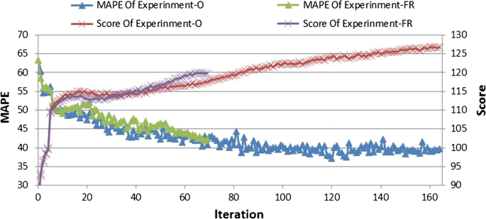
MAPEs and scores of each iteration in Experiment-FR and Experiment-O
-
(2)
Computing time For both Experiment-FR and Experiment-O, one of the stopping criteria is that the relative changes of averages score of executed plans should remain below 0.001 for four consecutive iterations. A model meeting this criterion is assumed to have converged: the non-converged model will stop automatically after the 500th iteration. The convergence of original and improved versions is also shown in Fig. 4. It can be seen that the improved MATSim converges at iteration 69, while the original MATSim converged at iteration 164. The computing time of Experiment-FR is 549 s, compared to1263 s for Experiment-O. This is due to the new replanning mechanism which only keeps those agents who are not satisfied with their current plans replanning. As the simulation continues, it should become more and more difficult for agents to find a better plan with a higher score. As a result, agents stop replanning sooner and the simulation converges more quickly.

According to the analysis above, the new framework and replanning module can significantly reduce the computing time (by about 50%) as a result of more rapid convergence, but with some sacrifice of model accuracy (the difference between original and improved MATSim in MAPE is about 3%). However, it should be noted that the maximum number of plans stored in the agents ‘memory (\( N_{Plans} \)) is set to 20. This may increase the demand on the computer’s RAM (Random Access Memory) and could be a challenge for very large-scale scenarios containing massive numbers of agents. Furthermore, \( N_{Plans} \) may be set with a smaller number, but one should bear in mind that this will result in a smaller number of candidate plans for reference when agents make decisions whether or not to continue replanning, and this will tend to make it more likely that agents end up in local optima, and more difficult for the simulator to find an overall global optimal solution.
Testing execution module (Experiment-E)
Similar to Experiment-FR, the Experiment-E is used to compare the performance of the new and original Execution Modules. Experiment-E is composed of two steps: (1) find the peak periods when the number of agents moving on the road network is large (2) assign different time step sizes to different periods. In this case study, in order to find a useful time step for the new execution module, the performance of the original MATSim was tested with steps ranging from 1 to 120 s (Fig. 5a). It can be seen that for the majority of simulations, the MAPEs do not change significantly after 300th iteration. Therefore, the maximum number of iterations can be set to 300 when applying the varying time-step based approach in this case study. Figure 5b shows the MAPEs of the last iterations, smallest MAPEs over iterations and computing time per iteration with time steps from 1 to 120 s. It can be seen that with the increase of the time step, the computing time per iteration heavily decreases for the first 15 iterations and then levels off at around 3 s after the 15th iteration. Both MAPEs of last iterations and smallest MAPEs over iterations have similar trends: the MAPE significantly decreases by about 20% for the first 50 iterations and then rises and fluctuates between 25 and 30%. In addition, it is worth noting that the MAPEs are larger for the smaller time steps in some cases: this seems strange, as the simulation with larger time step would be expected to lose more detail of agents’ movement, and thus decrease the model accuracy in terms of traffic flow. The main cause of this phenomenon could be the number of iterations required for simulation convergence, which is another factor significantly influencing the MAPEs in addition to the time step. Specifically, the smaller MAPEs are generally obtained with a larger number of iterations, shown by the simulations with time steps of 105 (500 iterations, MAPE of 25.51%), 50 (500 iterations, MAPE of 22.85%) and 40 (452 iterations, MAPE of 25.20%). This phenomenon is consistent with the iterative optimization concept of MATSim. Figure 5c shows the total numbers of iterations and total computing times of simulations with time steps ranging from 1 to 120 s. It can be seen that the number of iterations and total computing time seemingly do not have a monotonic variation with the time step, as with the increase of time step, the computing time and number of iteration can either increase or decrease. The reason is as follows: the change in time step is associated with the frequency of updating the status of each agent (e.g., location) in the simulation. However, the updating frequency tends to have no linear relationship with replanning behaviour of agents and further the resulting scores of each daily plan. As a result, the number of iterations needed to reach a stable point when the average score remains below 0.001 for four consecutive iterations would not have any significant (or linear) relationship with time step. For the total computing time, it is associated with both the number of iterations and computing time per iteration. Although the computing time per iteration only changes slightly when the time step is set above 20 s (see Fig. 5b), the total computing time is not linearly related with time step since the number of iterations needed varies with time step.

Computing times and accuracies of original MATSim with time steps from 1 to120
Based on the analysis above, time steps of 15 and 30 s were chosen for the Experiment-E, with a trade-off made between computing time and model accuracy. Specifically, with the increase of time step, the status of each agent will be updated less frequently and their moving trajectories will become less detailed. Therefore, we need to choose as smaller time steps as possible here. However, in order to pay equal attention to the total computing time, we choose 15 and 30 s as time step, as they tend to result in significantly shorter computing times (see Fig. 5c). In addition, the period from 7AM to 7PM is identified as the peak period because the number of agents moving on the road network is much larger and thus this period was allocated with time step 30: other periods were allocated with step 15.
As before, the performance of original and improved MATSim was compared in Table 1 in the following two aspects:
-
(1)
Model Accuracy: the MAPE of the improved MATSim in Experiment-E with varying time steps of 15 and 30 s is 30.49%, compared again to 37.48% for Experiment-O with time step of 1 s, and the MAPE in Experiment-E is just between those of original MATSim with steps of 15 and 30 s which are 31.62% and 25.40%, respectively; Similarly, the SD of the improved MATSim in Experiment-E is 20.48%, which is also between those of original MATSim with steps of 15 and 30 s which are 24.76% and 18.30%, respectively.
-
(2)
Computing Time: The computing time in Experiment-E is 652 s which is dramatically less than the one of 1187 s in Experiment-O. In addition, the computing time of Experiment-E with varying time steps of 15 and 30 s is just between those of original MATSim with steps of 15 and 30 which are 540 s and 684 s, respectively. In summary, in this case study, the new execution module can improve the performance of MATSim in both model accuracy and runtime in terms of car travel behavior simulation, compared with the original MATSim.
Testing combination of new modules (Experiment-C)
On the basis of the Experiment-FR and Experiment-E, Experiment-C was set up to test the overall performance of the improved MATSim that incorporates all new proposed methods including the new framework, new replanning module and new execution module. The performance of the improved MATSim in Experiment-C can be assessed through the comparison among four experiments, and the results are shown in Table 2. The comparison suggests that the improved MATSim in Experiment-C outperforms those in Experiment-FR and Experiment-E, as well as the original one in Experiment-O in terms of computing time. For model accuracy (measured with both MAPE and SD), Experiment-C performs better than Experiment-O and Experiment-FR, but slightly worse than Experiment-E. Specifically, the improved MATSim in Experiment-C takes less time (305 s) to converge, but obtains relatively good model accuracy with MAPE of 34.50% and SD of 25.15%, compared with Experiment-FR (Time of 549 s, MAPE of 42.45%, SD of 31.33%), Experiment-E (Time of 652 s, MAPE of 30.49%, SD of 20.48%) and Experiment-O (Time of 1187 s, MAPE of 42.13%, SD of 29.16%). In all, the improved MATSim incorporating all new modules can significantly reduce the computing time and get a relatively good accuracy.
Conclusions
An attempt is made to improve computing time in an integrated framework incorporating an activity-based model (ABM) with dynamic traffic assignment (DTA), using MATSim, a typical type of such integrated framework, as an example. The improvement work focused on two aspects: (1) the reduction of the number of iterations to converge (2) and the reduction of computing time for each iteration, with the application of a more focussed replanning algorithm and a varying time step approach in the execution module of MATSim. On the basis of the case study, it is found that both solutions are effective, at least for one rather specific case and choice of parameters. Specifically, for the first solution that reduces the number of iterations, the improved MATSim incorporating the new framework and replanning module can improve the original one in computing time at the cost of slight decrease in model accuracy; While, for the second solution that reduces the time of running each iteration, the varying time step based approach outperforms the original one in both computing time and model accuracy. However, the improved MATSim that incorporates all new improvement methods is able to simultaneously overcome the two limitations by combining the advantages of the new proposed methods.
Although the proposed improvement methods can significantly reduce the computing time and obtain a somewhat more accurate outcome, several issues remain to be studied. First, the improvement methods involve several new added parameters that are closely related to the effectiveness of the method. Currently, the parameters are set based on ad-hoc trials. However, it is important to fully investigate the sensitivity of the parameters and find a practical approach to optimally setting the parameters, so that MATSim can run at an optimal (or nearly best) speed, rather than just a faster speed, and to demonstrate more comprehensively that the proposed improvements are generally effective. Furthermore, as an integrated framework, MATSim contains a number of parameters from both ABM and DTA. This paper calibrated both the original and improved MATSim models with Cadyts by selecting optimal daily plans rather than estimating these parameters. It would be more behaviorally sound and accurate to calibrate the models through parameter estimation. However, this could be computationally infeasible or expensive, especially for large-scale scenarios, as such a calibration method needs to run the model many times with multiple parameter combinations. A further study is therefore in principle needed to see whether the improvements we suggest here (that refer mostly to the ABM part of the model) carry over into a more complete calibration of the entire MATSim model. Second, the new proposed framework and modules need to be tested within as many case studies as possible to further confirm its advantages in computing time and model accuracy. Especially for the very large-scale scenarios, such as Beijing and Shanghai, the computing time may be gained at the cost of using more memory, since more daily plans need to be stored in agents’ memory, and this could make the new proposed module infeasible. Furthermore, another way to test the improved model is to calibrate and validate it using different periods. For example, data collected during the morning and evening peak hours can be used for calibration and validation, respectively.
While the application here has been to MATSim specifically, similar considerations for improving model performance are likely to apply in other modeling frameworks. In particular using selective methods for reducing the number of agents active during computationally expensive routines (such as replanning) and varying the time step appropriately to the dynamics of the system may well be helpful. The non-monotonic behavior of the original code with time step suggests that understanding the way the non-linear dynamics of the models is behaving could be an aid in finding places where such time step changes could be expected to be useful.
References
Auld, J., Mohammadian, A.: Framework for the development of the agent-based dynamic activity planning and travel scheduling (ADAPTS) model. Transp. Lett. 1(3), 245–255 (2009)
Axhausen, K.W.: Agent-based modelling of travel behaviour and flow: the MATSim implementation in Singapore and elsewhere. In: Seminar of Hong Kong Society for Transportation Studies and The Hong Kong Polytechnic University, Hong Kong, China (2013)
Balmer, M.: Travel demand modeling for multi-agent transport simulations: algorithms and systems, Doctoral Dissertation, ETH Zurich, Swizerland (2007)
Balmer, M., Meister, K., Rieser, M., Nagel, K., Axhausen, K.W.: Agent-based simulation of travel demand: structure and computational performance of MATSim-T. ETH, Eidgenössische Technische Hochschule Zürich, IVT Institut für Verkehrsplanung und Transportsysteme, Zürich (2008)
Balmer, M., Rieser, M., Meister, K., Charypar, D., Lefebvre, N., Nagel, K., Axhausen, K.: MATSim-T: Architecture and simulation times. In: Multi-Agent Systems for Traffic and Transportation Engineering, pp. 57–78 (2009)
Bekhor, S., Dobler, C., Axhausen, K.W.: Integration of activity-based with agent-based models: an example from the Tel Aviv model and MATSim. ETH Zürich, Institut für Verkehrsplanung, Transporttechnik, Strassen-und Eisenbahnbau (IVT), Zürich (2010)
Bellemans, T., Kochan, B., Janssens, D., Wets, G., Arentze, T., Timmermans, H.: Implementation framework and development trajectory of FEATHERS activity-based simulation platform. Transp. Res. Rec. J. Transp. Res. Board 2175(1), 111–119 (2010)
Bradley, M., Bowman, J.L., Griesenbeck, B.: SACSIM: an applied activity-based model system with fine-level spatial and temporal resolution. J. Choice Model. 3(1), 5–31 (2010)
Brinckerhoff, P.: San Francisco dynamic traffic assignment project “DTA Anyway”: final methodology report. San Francisco County Transportation Authority, San Francisco, Calif (2012)
Castiglione, J., Bradley, M., Gliebe, J.: Activity-based travel demand models: a primer. The National Academies Press, Washington, DC (2015)
Castiglione, J., Grady, B., Bowman, J., Bradley, M., Lawe, S.: Building an integrated activity-based and dynamic network assignment model. In: 3rd Transportation Research Board Conference on Innovations in Travel Modeling, Tempe, Ariz (2010)
Charypar, D., Axhausen, K., Nagel, K.: Implementing activity-based models: accelerating the replanning process of agents using an evolution strategy. In: 11th International Conference on Travel Behaviour Research, Kyoto (2006)
Charypar, D., Axhausen, K.W., Nagel, K.: An Event-Driven Parallel Queue-Based Microsimulation for Large Scale Traffic Scenarios. ETH, Eidgenössische Technische Hochschule Zürich, IVT, Zürich (2007)
Dobler, C.: Implementation of a time step based parallel queue simulation in MATSim. In: 10th Swiss Transport Research Conference. Monte Verita, Ascona (2010)
Flötteröd, G.: Cadyts-A free calibration tool for dynamic traffic simulations. In: 9th Swiss Transport Research Conference, Ascona, Switzerland (2009)
Flötteröd, G., Bierlaire, M., Nagel, K.: Bayesian demand calibration for dynamic traffic simulations. Transp. Sci. 45(4), 541–561 (2011)
Flötteröd, G., Chen, Y., Nagel, K.: Behavioral calibration and analysis of a large-scale travel microsimulation. Netw. Spat. Econ. 12(4), 481–502 (2012)
Fourie, P., Illenberger, J., Nagel, K.: Increased convergence rates in multiagent transport simulations with pseudosimulation. Transp. Res. Rec. J. Transp. Res. Board 2343, 68–76 (2013)
Gao, W., Balmer, M., Miller, E.: Comparison of MATSim and EMME/2 on greater Toronto and Hamilton area network, Canada. Transp. Res. Rec. J. Transp. Res. Board 2197, 118–128 (2010)
Hadi, M., Pendyala, R., Bhat, C., Waller, T.: Dynamic, Integrated Model System: Jacksonville-Area Application. Transportation Research Board of the National Academies, Washington, D.C. (2014)
Horni, A., Nagel, K., Axhausen, K.W.: The Multi-Agent Transport Simulation MATSim. Ubiquity, London (2016)
Horni, A., Scott, D., Balmer, M., Axhausen, K.: Location choice modeling for shopping and leisure activities with MATSim: combining microsimulation and time geography. Transp. Res. Rec. J. Transp. Res. Board 2135, 87–95 (2009)
Javanmardi, M., Auld, J., Mohammadian, A.K.: Integration of TRANSIMS with the ADAPTS activity-based model. In: Fourth TRB Conference on Innovations in Travel Modeling (ITM), Tampa, FL (2011)
Kitamura, R., Fujii, S., Yamamoto, T., Kikuchi, A.: Application of PCATS/DEBNetS to regional planning and policy analysis: micro-simulation studies for the cities of Osaka and Kyoto, Japan. In: Proceedings of Seminar F of the European Transport Conference 2000, Cambridge, United Kingdom (2000)
Kitamura, R., Kikuchi, A., Fujii, S., Yamamoto, T.: An overview of PCATS/DEBNetS micro-simulation system: its development, extension, and application to demand forecasting. In: Kuwahara, M. (ed.) Simulation Approaches in Transportation Analysis, pp. 371–399. Springer, Berlin (2005)
Kitamura, R., Kikuchi, A., Pendyala, R.: Integrated, dynamic activity-network simulator: current state and future directions of PCATS-DEBNetS. In: Presentation at the Second TRB Conference on Innovations in Travel Modeling, Portland, OR, June, pp. 22–24 (2008)
Lefebvre, N., Balmer, M.: Fast Shortest Path Computation in Time-Dependent Traffic Networks. ETH, Eidgenössische Technische Hochschule Zürich, IVT, Institut für Verkehrsplanung und Transportsysteme, Zürich (2007)
Lin, D.-Y., Eluru, N., Waller, S.T., Bhat, C.R.: Integration of activity-based modeling and dynamic traffic assignment. Transp. Res. Rec. J. Transp. Res. Board 2076(1), 52–61 (2008)
Maciejewski, M., Nagel, K.: Simulation and dynamic optimization of taxi services in MATSim, VSP Working Paper 13-05, TU Berlin, Transport Systems Planning and Transport Telematics (2013)
MATSim:. Scenarios of MATSim. Retrieved 31 May 2015 from http://www.matsim.org/scenarios (2015)
Meister, K., Balmer, M., Ciari, F., Horni, A., Rieser, M., Waraich, R.A., Axhausen, K.W., Waraich, R.A., Waraich, R.A., Axhausen, K.W.: Large-Scale Agent-Based Travel Demand Optimization Applied to Switzerland, Including Mode Choice. ETH, Eidgenössische Technische Hochschule Zürich, IVT, Institut für Verkehrsplanung und Transportsysteme, Zürich (2010)
Nagel, K., Flotterod, G.: Agent-based traffic assignment. In: Horni, A., Nagel, K., Axhausen, K.W. (eds.) The Multi-Agent Transport Simulation MATSim, pp. 315–326. Ubiquity, London (2016)
National Academies of Sciences, Engineering, and Medicine: Dynamic, Integrated Model System: Sacramento-Area Application, Volume 1: Summary report. The National Academies Press, Washington, DC (2014)
Neumann, A., Balmer, M., Senozon, A., Rieser, M.: Converting a static macroscopic model into a dynamic activity-based model to analyze public transport demand in Berlin. In: IATBR 2012 (2012)
Neumann, A., Röder, D., Joubert, J.W.: Towards a simulation of minibuses in South Africa. J. Transp. Land Use 8(1), 137–154 (2015)
Pendyala, R.M., Konduri, K.C., Chiu, Y.-C., Hickman, M., Noh, H., Waddell, P., Wang, L., You, D., Gardner, B.: Integrated land use-transport model system with dynamic time-dependent activity-travel microsimulation. Transp. Res. Rec. J. Transp. Res. Board 2303(1), 19–27 (2012)
Pinjari, A., Eluru, N., Srinivasan, S., Guo, J.Y., Copperman, R., Sener, I.N., Bhat, C.R.: Cemdap: Modeling and microsimulation frameworks, software development, and verification. In: TRB 87th Annual Meeting Compendium of Papers DVD. Washington DC, pp. 13–17 (2008)
Röder, D., Cabrita, I., Nagel, K.: Simulation-based sketch planning, part III: calibration of a MATSim-model for the greater Brussels area and investigation of a cordon pricing for the highway ring, VSP working paper 13-16, TU Berlin, Berlin, Germany (2013)
Ramaekers, K., Kochan, B., Bellemans, T., Janssens, D., Wets, G.: Linking activity-based travel demand models and traffic assignment: a Flemish case study. In: Innovations in Travel Modelling, Portland, U.S.A (2008)
Rasouli, S., Timmermans, H.: Activity-based models of travel demand: promises, progress and prospects. Int. J. Urban Sci. 18(1), 31–60 (2014)
Rieser, M.: Adding Transit to an Agent-Based Transportation Simulation. Technische Universität Berlin, Berlin, Doctoral Disseration (2010)
Smith, L., Beckman, R., Anson, D., Nagel, K., Williams, M.E.: TRANSIMS: Transportation analysis and simulation system. In: Fifth National Conference on Transportation Planning Methods Applications, Seattle, Washington (1995)
Waller, S., Ziliaskopoulos, A.: A visual interactive system for transportation algorithms. In: 78th Annual Meeting of the Transportation Research Board, Washington, DC (1998)
Waraich, R.A., Charypar, D., Balmer, M., Axhausen, K.W.: Performance improvements for large-scale traffic simulation in MATSim. In: Helbich, M., Leitner, M. (eds.) Computational Approaches for Urban Environments, pp. 211–233. Springer, Berlin (2015)
Waraich, R.A., Galus, M.D., Dobler, C., Balmer, M., Andersson, G., Axhausen, K.W., Waraich, R.A., Waraich, R.A., Andersson, G., Andersson, G.: Plug-in Hybrid Electric Vehicles and Smart Grid: Investigations Based on a Micro-simulation. ETH, Eidgenössische Technische Hochschule Zürich, IVT, Institut für Verkehrsplanung und Transportsysteme, Zürich (2009)
Zhang, L., Yang, W., Wang, J., Rao, Q.: Large-scale agent-based transport simulation in Shanghai, China. Transp. Res. Rec. J. Transp. Res. Board 2399(1), 34–43 (2013)
Zhuge, C.: Dynamic evolution mechanism of urban transport-land use based on self-organizing theory. Doctoral Dissertation, Beijing Jiaotong University, China (2014)
Zhuge, C., Li, X., Ku, C.-A., Gao, J., Zhang, H.: A heuristic-based population synthesis method for micro-simulation in transportation. KSCE J. Civ. Eng. 21(6), 2373–2383 (2017)
Zhuge, C., Shao, C.: Baoding: a case study for testing a new household utility function in MATSim. In: Horni, A., Nagel, K., Axhausen, K.W. (eds.) The Multi-agent Transport Simulation MATSim, pp. 409–412. Ubiquity, London (2016)
Zhuge, C., Shao, C., Gao, J., Meng, M., Xu, W.: An initial implementation of multiagent simulation of travel behavior for a medium-sized city in China. Math. Probl. Eng. 2014, 1–11 (2014)
Ziemke, D., Nagel, K., Bhat, C.: Integrating CEMDAP and MATSim to increase the transferability of transport demand models. Transp. Res. Rec. J. Transp. Res. Board 2493, 117–125 (2015)
Acknowledgements
This research was supported by the National Natural Science Foundation of China (Grant Numbers 51678044; 71401012), the Fundamental Research Funds for the Central Universities (NO. 2017JBZ106), China, the Hong Kong Polytechnic University [1-BE2 J], the Hebei Natural Science Foundation (Grant Number E2016513016) and ERC Starting Grant #678799 for the SILCI project (Social Influence and disruptive Low Carbon Innovation). This paper was also presented on the 14th World Conference on Transport Research.
Author information
Authors and Affiliations
Contributions
CZ: Literature Search and Review, Case Study, Modelling and Computing, and Manuscript Writing; MB: Manuscript writing and Editing, Case Study, and Modelling; CS: Modelling, Case Study and Manuscript Editing; XL: Modelling and Manuscript Editing; JG: Data Preparation and Manuscript Editing
Corresponding authors
Ethics declarations
Conflict of interest
The authors declare that they have no conflict of interest.
Additional information
Publisher's Note
Springer Nature remains neutral with regard to jurisdictional claims in published maps and institutional affiliations.

Rights and permissions
Open Access This article is distributed under the terms of the Creative Commons Attribution 4.0 International License (http://creativecommons.org/licenses/by/4.0/), which permits unrestricted use, distribution, and reproduction in any medium, provided you give appropriate credit to the original author(s) and the source, provide a link to the Creative Commons license, and indicate if changes were made.
About this article

Cite this article
Zhuge, C., Bithell, M., Shao, C. et al. An improvement in MATSim computing time for large-scale travel behaviour microsimulation. Transportation 48, 193–214 (2021). https://doi.org/10.1007/s11116-019-10048-0
Published:
Issue Date:
DOI: https://doi.org/10.1007/s11116-019-10048-0